Similar artist network

Motivation

If you are anything like me, you occasionally find yourself coming up for air after a long diversion clicking through artist biographies on Spotify. Often these biographies will list the artists other bands or people they have played with, and one thing leads to another and I have added twenty albums to my “new music” playlist folder.

I found myself in this position one morning after listening to this episode of Casual Inference, a great podcast that has unfortunately gone radio silent of late. The guest, Betsy Ogburn, is an expert in causality in social networks, a difficult (so. much. endogeneity.) and super interesting field. I had been reading one of her papers and so my brain was primed for thinking about networks. Could I use the Spotify API to create an artist network to investigate questions like:

• Does having a more popular artist guest on a track garner more listens?
• Does having a certain producer increase listens?
• Do super studio musicians have any effect on track plays?

I quickly discovered that this is unfortunately not one of the endpoints in the amazing Spotify API (go check it out if you never have)¹. After inquiring about this absence, I realized that the “Related artists” are a natural way to build an artist network.

Prior to this I had never done any network analysis with python, so I thought this could be an interesting way to interact with Spotify’s API in a new way and learn a little bit about what python tools are available for network analysis. This is my “what can I do in an hour” exploration of these ideas.

Cleanup

Disclaimer: This post is a quick and dirty analysis! My time was limited, so basically I constrained myself to seeing if I could figure out the relevant tooling and make a plot. I have left it messy so you can see my process getting from nothing to something at least marginally interesting.

I am not including the code to pull the artist information from Spotify. If you are interested, the code for that is on github here. I saved it as json, so the first thing I do here is import the packages I will use in the analysis and massage the data into the shape I need to plot the network. Networkx seems to be the main python package for network analysis in python. I barely scratch the surface here.

import json

import networkx as nx
import pandas as pd
import numpy as np


# load artist data
with open('../data/raw/followed_artists.json') as f:
    artists = json.load(f)

Spotify includes a lot of metadata and other information that I am not interested in for this exercise, so the next cell makes a dictionary of only the data that is relevant for my purposes.

# create a dictionary of the relevant information
artists_dict = {}
artists_dict['id'] = [i['id'] for i in artists]
artists_dict['artist'] = [i['name'] for i in artists]
artists_dict['followers'] = [i['followers']['total'] for i in artists]
artists_dict['popularity'] = [i['popularity'] for i in artists]
artists_dict['related_artist'] = [i['related_artists'] for i in artists]

Pandas has a bunch of different methods for reading data into dataframes. .from_dict() will take a dicitonary as input and create a dataframe

df = pd.DataFrame.from_dict(artists_dict)

Now we have a dataframe we can use with NetworkX. Unfortunately, the related_artist column is a list. I need to expand it so that each item in the list gets it’s own row along with all of the other data in that row. This was a trickier problem that I initially anticipated, but thankfully someone before me had the same problem and a stackoverflow samaritan came to their rescue.

# "melt" name list into individual rows
# https://stackoverflow.com/questions/27263805/pandas-column-of-lists-create-a-row-for-each-list-element

lst_col = 'related_artist'

r = pd.DataFrame({
      col:np.repeat(df[col].values, df[lst_col].str.len())
      for col in df.columns.drop(lst_col)}
    ).assign(**{lst_col:np.concatenate(df[lst_col].values)})[df.columns]

Unfortunately, it turns out A$AP Rocky and Joey Bada$$ are too bada$$ for NetworkX.

r.loc[r['related_artist'].str.contains('\$')]

.dataframe tbody tr th {
    vertical-align: top;
}

.dataframe thead th {
    text-align: right;
}

The $ is a special character and breaks the graphing algorithm. I will make them significantly less cool by replacing their $ with S.

# temp fix to remove special characters from name (Joey Bada$$ and A$AP Rocky were throwing errors)
r['artist'] = r['artist'].str.replace('$', 'S')
r['related_artist'] = r['related_artist'].str.replace('$', 'S')
r.loc[r['related_artist'].str.contains('\$')]

.dataframe tbody tr th {
    vertical-align: top;
}

.dataframe thead th {
    text-align: right;
}

There we go. On to the network graph!

Visualization

NetworkX provides a very user friendly out of the box graphing method that will allow you to get a sense of the basic structure of a graph. It is essentially just a wrapper around matplotlib, so you can use matplotlib’s extensive (and often arcane) customization if you need to make something pretty to show your bosses. For my current purposes, I just want to get a sense of the network structure, then go on to look at some of the statistical features of the network. Here goes.

G = nx.from_pandas_edgelist(r, 
                            source='artist',
                            target='related_artist',
                            edge_attr='followers',
                            create_using=nx.DiGraph())

nx.draw_networkx(G)

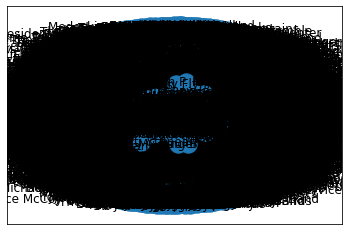
Oof, that’s not very helpful. It looks like it could be a bit donut shaped? Let’s pare things down a bit. I’m just going to take a random sample and replot to see if that helps.

r_graph = r.sample(100)
G = nx.from_pandas_edgelist(r_graph, 
                            source='artist',
                            target='related_artist',
                            edge_attr='followers',
                            create_using=nx.DiGraph())

nx.draw_networkx(G)

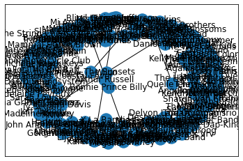
There’s our donut! It’s definitely a small world graph with a few artists in the middle, connecting the disparate groups (makes sense that Arthur Russell and Bonnie Prince Billy would be the weirdos crossing over :).

Let’s get rid of the names, make the nodes smaller and increase the sample size a bit.

r_graph = r.sample(500)
G = nx.from_pandas_edgelist(r_graph, 
                            source='artist',
                            target='related_artist',
                            edge_attr='followers',
                            create_using=nx.DiGraph())

nx.draw_networkx(G, with_labels=False, node_size=10)

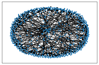
Much better. Just lighten up the edges a touch and…

nx.draw_networkx(G, with_labels=False, node_size=10, width=0.5)

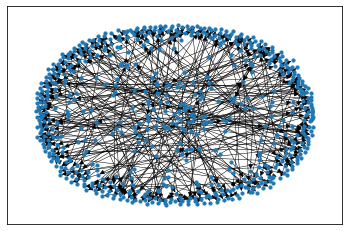
Voila!

Is this a Small World Network?

Visually, this looks like it could be a Small-world network, with a sort of halo of clusters around the edgo of the graph and a non-trivial number of paths from opposing edges. From the Wikipedia article:

A small-world network is a type of mathematical graph in which most nodes are not neighbors of one another, but the neighbors of any given node are likely to be neighbors of each other and most nodes can be reached from every other node by a small number of hops or steps.

To wrap up this blog post, I am going to calculate some statistics to see if this indeed is likely a Small-world network and have a look at the artists that most connect otherwise disparate parts of the graph.

One of the signature characteristics of this type of network is that the distance between randomly chosen nodes (in this case artists) is proportional to the logarithm of the total number of nodes in the network².

According to this post, the best way to do this is to calculate the mean shortest path length and clustering coefficients of your network and compare them to the equivalent statistics of a synthetic random network. So this is what we will do. But before we do that, let’s talk about what exactly those things are.

Diversion on path length and clustering

TODO: briefly explain clustering and path length

Now, back to our analysis. Our procedure is the following:

1. Calculate average path length and clustering coefficient of the original network.
2. Generate the appropriate synthetic network.
3. Repeat Step 1 for the synthetic network.
4. Calculate small-world statistics.
5. Prosper.

Why do we care about whether or not this is a small world network?

The network we are examining is all of the related artists of the artists I follow on Spotify. What is this, exactly? According to the Spotify API docs, related artists are artists similar to a given artist and similarity is based on analysis of the Spotify community’s listening history. This article goes into a bit more detail, hinting that size of listenership and number of shared listeners are important parameters in the algorithm that decides shared listeners, but few details are provided. This means that at a high, hand-wavy level, the related artists I see for Benny Sings are just other artists whose listeners overlap in some significant way with Benny Sings’ listeners.

So what we have here is a listening network.

Questions:

• Who is connected to the most other artists?
• Who connects otherwise poorly connected regions?
• Do we have any natural clusters or communities? What do they have in common?